Project
TeneaX
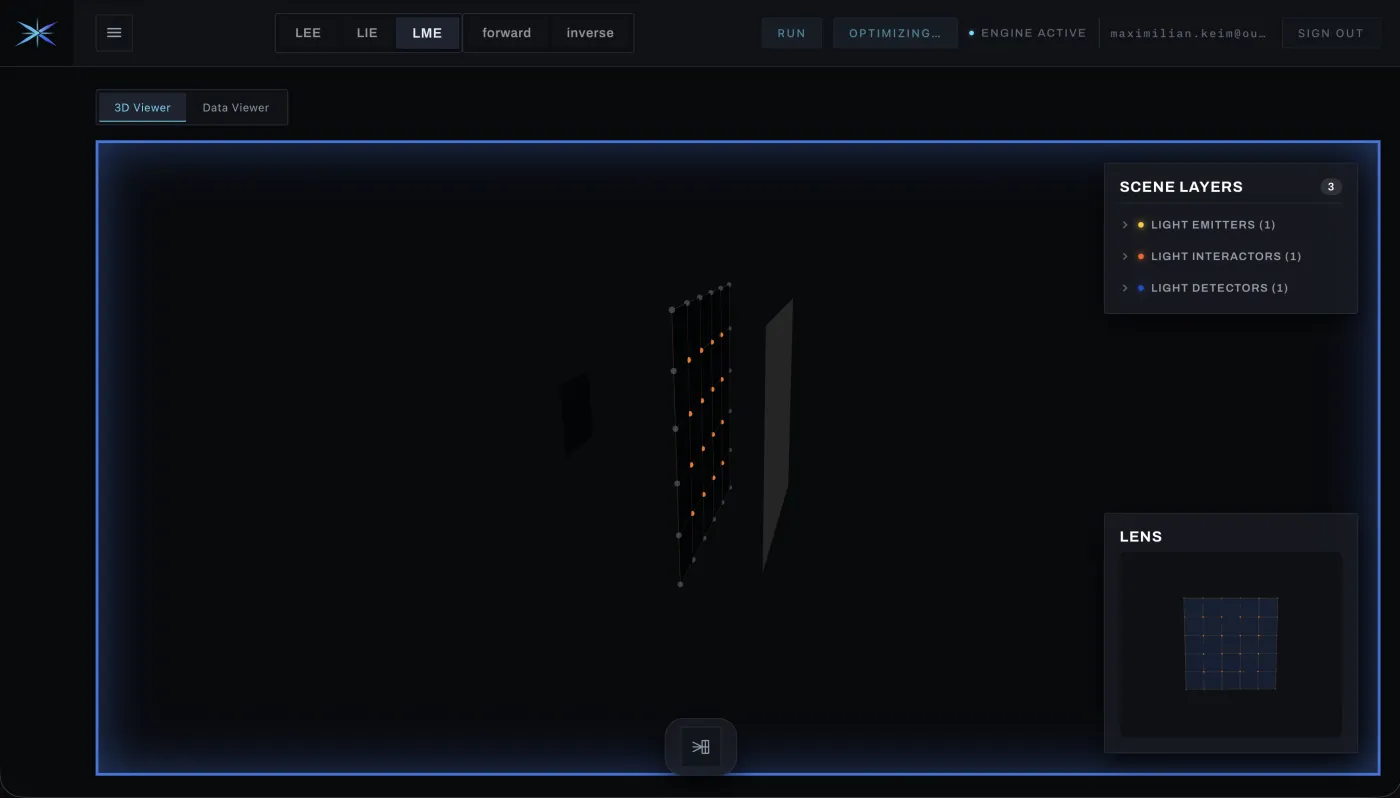
TeneaX is an inverse optical design engine. Classical lens design is a forward, trial and error loop: you shape a surface, trace the light, look at the result, and adjust. TeneaX aims to invert that. You specify the illuminance pattern you want on a target plane, and the engine solves for the lens that produces it, automatically, by gradient based optimization. Formally it minimizes the mismatch between the achieved and the target distribution, where are the control points of a freeform lens and is the illuminance from tracing thousands of rays through it.
Ray Tracing
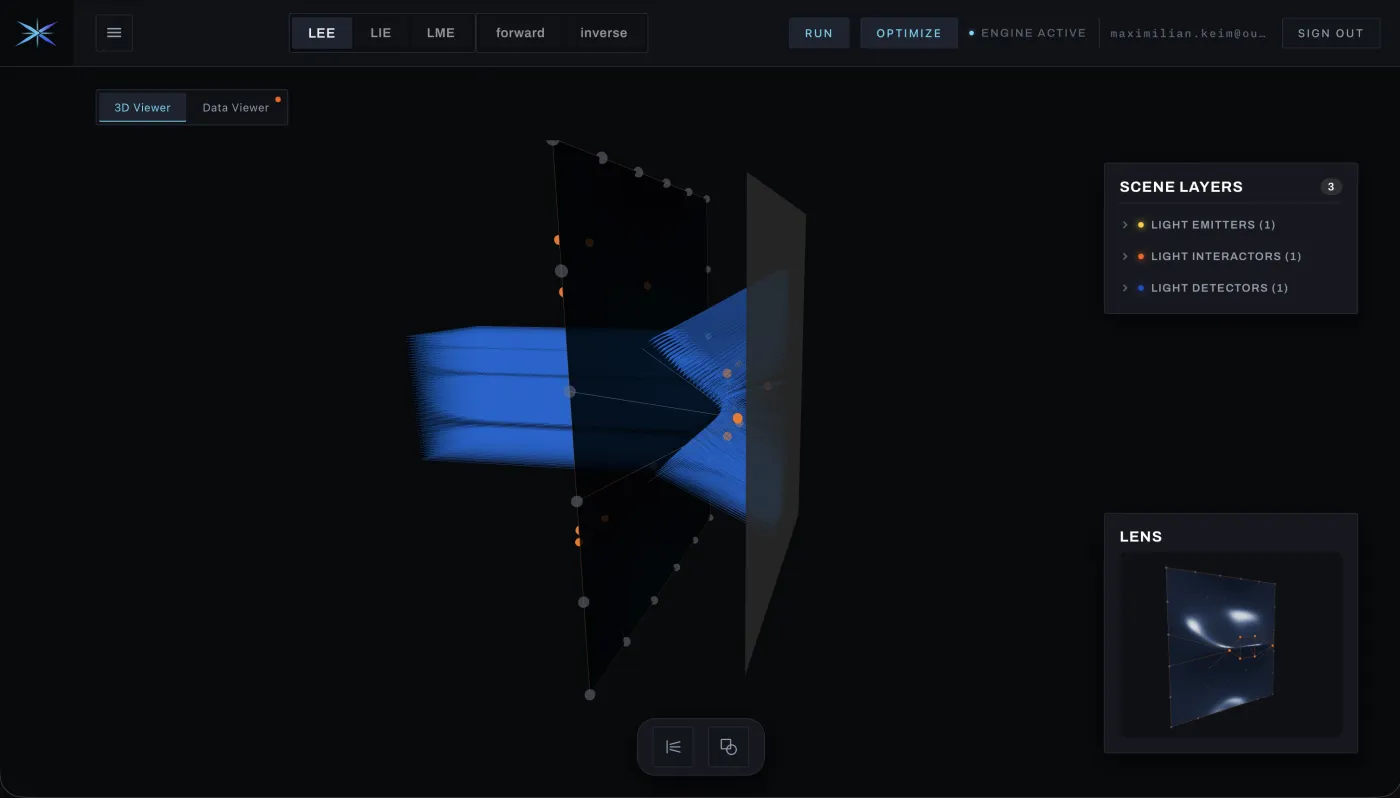
At the heart of TeneaX is a physically based ray tracer. Thousands of rays are emitted from the source, refracted through the freeform lens, and accumulated on a detector to form the illuminance image that the optimizer scores. The physics is standard: each ray refracts by the vectorial Snell's law with and . Getting this forward model right, and numerically robust through total internal reflection and grazing incidence, is what makes the whole inverse design loop trustworthy.
NURBS Surfaces
The lens surface has to be smooth, freeform, and controllable with a manageable number of parameters, which is exactly what a NURBS surface gives you. It is a weighted combination of B-spline basis functions over a grid of control points, where the control points are the design variables the optimizer moves and everything else stays fixed. A modest grid already spans a rich space of freeform shapes while keeping the problem well conditioned. Tracing a ray against such a surface has no closed form, so every intersection is found by Newton-Raphson iteration, solving for .
Resulting Surface
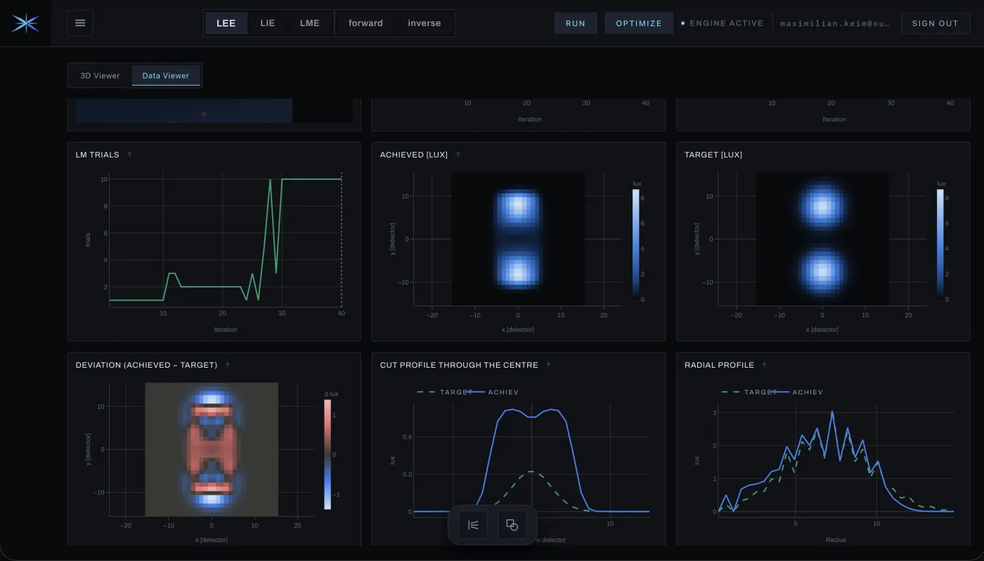
With the forward model and a NURBS parametrization in place, the inverse problem becomes a least squares fit, and the classic optical design optimizer applies: Levenberg-Marquardt. Writing the merit as residuals , each step solves and moves the control points by . The damping interpolates between Gauss-Newton (fast, ) and gradient descent (safe, ): a step is accepted only if it lowers the cost, otherwise is raised and the step retried. That single rule also makes the solver robust to the numerical pathologies of ray tracing, such as total internal reflection and grazing hits, that would otherwise poison the optimization. The goal is a freeform lens, expressed in real photometric units (Lux), that reshapes the source into the specified target pattern.